This tech tip was heavily informed by Ed Janowiak’s past symposium presentations. You can watch his presentation about setting proper airflow HERE. You can also now purchase your tickets for the 6th Annual HVACR Training Symposium HERE.

HVAC School was founded by a Floridian—representing Climate Zone 2, to be exact. So, it’s no surprise that “humid climate” markets and their unique needs come up an awful lot on this platform. For example, proper equipment sizing is an absolute must if we want to combat the climate's mugginess. 

While relative humidity (or RH) is what most likely comes to mind when we think of humidity, it actually doesn’t mean that much from a design standpoint. Sure, we have indoor RH targets, but dew point tends to be a more telling factor when it comes to distinguishing what makes a “humid,” “green-grass,” or “dry” market in terms of system design. 

However, that’s also tricky because there’s not a clear line we can draw across the USA to separate those markets. Sizing and setting airflow are NOT as simple as figuring out which climate you’re in and ballparking your designs.

Review of the Dew Point

The dew point is the temperature at which the RH is 100%, This temperature will vary depending on the amount of moisture in the air. 

Think about how sugar dissolves more easily into hot tea than cold tea. The sugar mixes more easily into the hot tea, whereas it sinks to the bottom in cold tea. Moisture in the air follows a similar principle; hot air holds a lot of moisture, and cold air doesn’t.

The sugar at the bottom of a glass or cup of tea is like liquid water. On a dewy morning, the air temperature is below the dew point, so excess moisture is wrung out of the air and forms liquid dewdrops on surfaces like plants and cars.

In dry climates, you need rather cold temperatures before this phenomenon can happen. Since this tech tip was written in the spring, we’ll use a late May day as an example:

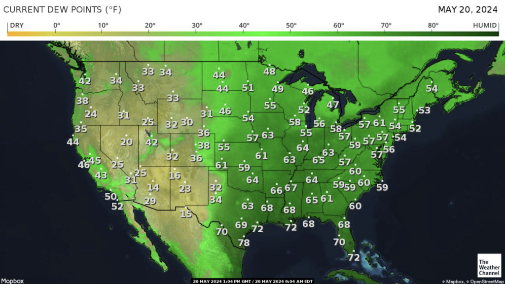
In much of the Southwest and Rocky Mountains, those temperatures are below freezing. In Florida, the dew point is around room temperature. It’s pretty easy to see what would count as a “humid climate,” a “green grass climate,” and a “dry climate.” The Southeast and even up through the Midwest and Northeast are all green, and much of the West is tan. But where do we draw the actual line?

Where’s the Boundary?

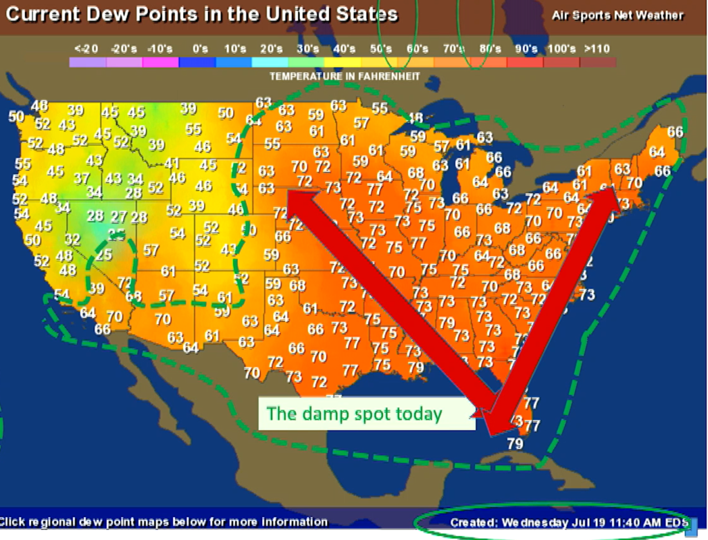
The dew point is dynamic; it doesn’t stay the same all the time. Since we have more precipitation and hotter weather in the summer, we can expect to see high dew points over a larger area, not just in that dark green Southeastern pocket shown above. 

In Ken Gehring, Andy Ask, and Nikki Krueger’s 2023 HVACR Training Symposium presentation, they showed the dew points across the contiguous U.S. on July 19th, 2022, and September 22, 2022, respectively.

The closest thing we might have to a hard line between “humid” and “dry” markets is Figure A10-4 from Version 2 of the Climate Atlas of the United States. 

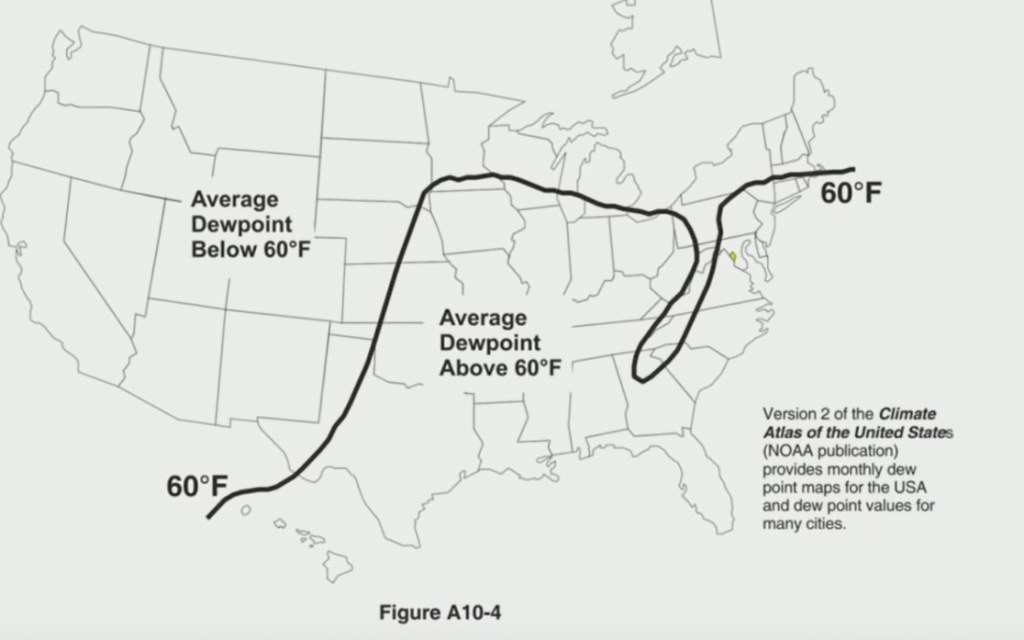
However, as you can see from the previous dew point maps, areas like northern Minnesota and Upstate New York are still capable of experiencing high dew points in the fall and spring, even if they are above that boundary. 

So, we can’t let location and a simplified understanding of dew points dictate our approach to sizing. Instead, let’s look at design goals and go from there.

Design Goals

Let’s remember that the ACCA design conditions in Manual J are based on historical climate data. We’d consult Table 1A for climate data from several airports and weather stations across the country.

We size equipment based on the temperature that will be exceeded 99% of the time in the winter. For example, based on historical data from the Orlando International Airport, that number would be 42°F. In the summer, we size equipment based on the temperature that will be exceeded 1% of the time. Using our same example, that would be 92°F. We do see temperatures in the 30s and upper 90s in Central Florida, but it’s not a regular thing, and we don’t want to size equipment based on anomalies. We want it to be able to heat and cool sufficiently for the majority of the time. If we’re designing for those fringe scenarios, then we’re more likely to encounter issues with part-load conditions.

Typical design goals will look something like this:

• Winter: 70°F at design conditions
• Summer: 75°F at design conditions, 50% RH (Indoor 62.5°F wet-bulb)

Of course, customers may have different goals—that’s on them. But the design conditions give us a pretty reliable guide, even though they’re not perfect.

Equipment Sizing Misconceptions

The ACCA Design manuals are meant to be used as a series. You don’t just use Manual J and call it a day; the equipment design also relies on Manuals S, D, and T to optimize comfort for your client. Blower speeds and equipment selection are a huge part of the process and cannot be overlooked.

Manual S isn’t as important for heating-only markets since the HVAC can only add sensible BTUs. An oversized heating system in these markets won’t pose the same problems that an oversized cooling system would. You have a decent amount of leeway on the heating-only side; Manual S allows oversizing up to 40%. 

However, anytime we have to factor cooling into the design, especially latent BTU removal, accurate equipment sizing becomes so much more important—and restrictive. Rules of thumb, like 400 CFM per ton, just don’t cut it. (Also, keep in mind that a 2-ton unit’s nominal capacity may be 24,000 BTUs per hour, but it’s almost certainly not going to deliver that due to various efficiency losses.)

We need to look at each situation on a case-by-case basis, not just based on location or nominal tonnage alone. We also don’t want to assume that variable-speed equipment can compensate for oversizing; the N2 section of Manual S states that you can’t oversize single-stage heat pumps by more than 15%, but that figure only bumps up to 20% and 30% for two-stage and variable-speed equipment, respectively. (There IS an exception to these rules, which we’ll cover later.) Variable-speed systems are NOT infinitely variable.

Instead of relying on rules of thumb and variable-speed equipment to cover those rules’ margins for error, we need to do the math. What we should really be focusing on is the sensible heat ratio (SHR and sensible heat factor or SHF), expanded performance data, and ACCA design processes.

Sensible Heat Ratio (SHR) and Sensible Heat Factor (SHF)

The SHR is the ratio of how many cooling BTUs are being used to move sensible heat, not latent heat. (SHR usually refers to the structure’s sensible to latent BTU ratio; when applied to equipment, this ratio is usually called sensible heat factor or SHF.) Sensible heat is heat that we can feel; it’s what we mean when we talk about temperature. Latent heat is hidden heat and has to do with the moisture load; it’s what we mean when we talk about humidity.

The SHR and SHF max out at 1, and higher numbers mean that the equipment is moving more sensible heat. For example, a system moving 10,000 BTUs of heat may be moving 9,400 sensible BTUs and 600 latent BTUs. That SHF will be 0.94, which is what we’d expect of a lot of high-efficiency ductless systems nowadays (which are great for energy savings but don’t tend to be as great at dehumidification).

We have to keep in mind that the structure and the equipment have different values. The SHR of a structure is the ratio of sensible BTUs that need to be moved, and the SHF of the equipment is the ratio of sensible BTUs being moved. It would be great if they matched—or had some excess latent BTU removal in humid climates.

We can manipulate SHF with fan speeds. When we have higher fan speeds, like 450 CFM per ton as opposed to 350 CFM per ton, we move more sensible BTUs over the coil and get more bang for our buck from an efficiency standpoint. But efficiency doesn’t help when we have latent BTUs to account for. When the blower is rushing air over that coil, there isn’t enough time for the cold coil to wring all that moisture out of the air. Sure, it’s moving more sensible BTUs, but it’s not doing much to take latent BTUs out of the equation.

Expanded Performance Data

When it comes to equipment sizing, using tonnage alone is a shortcut that doesn’t account for the big picture. The nominal tonnage will almost never match the actual tonnage, so that’s where the expanded performance data comes in handy.

The expanded performance data helps us look at the CFM, condenser entering air temperature, and total and sensible capacities. Lower blower speeds result in lower total and sensible capacity, and the SHF is decreased. However, when we use the SHF equation, we can tell that the latent capacity improves. That’s evident in the chart below.

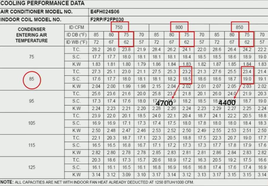
In the table above, the TC is the total capacity, and the SC is the sensible capacity. 

Building Tightness and Sizing

As many of you are familiar with at this point, homes have been getting tighter and tighter due to changing construction codes. “Leaky” homes have more opportunities for latent BTUs to infiltrate the space. (Remember: high humidity will go to low humidity. Humid air from an unconditioned attic or crawl space can seep into the conditioned space through gaps, such as those around recessed light fixtures.)

Tight homes with low latent loads (such as from a low number of occupants) are going to have high SHR values, and the equipment sizing will differ just a little. Remember our N2 restrictions? That our equipment selection can’t exceed 15, 20, or 30% of the load on single, two, and variable-speed systems? We can throw that out the window when a structure has an SHR exceeding 0.95. That is a very tight structure, and the rule is that we can’t oversize the equipment by more than 15% across all types—single, two, or variable-speed—when the structure SHR is greater than or equal to 0.95. 

Using Math for Equipment Sizing and Airflow

Arid climates don’t have to worry about latent loads very much at all (except in special circumstances, which we’ll get into later). But as long as we have humid or “green-grass” climate conditions, humidity control will be a design consideration when sizing equipment. 

You can start off by taking the BTU values from the expanded performance data; we want to look for the BTU output corresponding to the temperature of the outdoor air entering the condenser for design conditions. (Remember: consult Table 1A in Manual J for those values.) 

Since the data provides the total and sensible capacities, you can subtract the sensible capacity from the total to get the latent capacity (in BTUs). Divide the sensible capacity by the total capacity to get the equipment SHF. 

Interpolation

In many cases, the extended performance data shows the temperature of the outdoor air entering the condenser in increments of 10 with numbers that end in 5 (e.g., 75 and 85). However, 90°F is a common summer design condition across the country, but the expanded performance data above gives us 85°F and jumps straight to 95°F. So, how do we figure out what BTU loads we need to size for? 

That’s where interpolation comes in.

“Interpolation” is a fancy way of saying, “Add the numbers and then divide by two.” You’re finding the average between 85°F and 95°F. You would take the total capacity (in BTUs), add them, and divide by two to get the BTUs for 90°F. From there, you would do the same for the sensible capacity and can figure out the latent BTUs and equipment SHF based on those values. 

Find the Structure SHR

Previously, Manual J recommended using 350 CFM for homes with SHRs of around 0.70, 400 CFM for 0.80, and 450–500 CFM for 0.90+. Nowadays, we’re supposed to take the structure SHR we receive from our Manual J load calculation and compare it to the math we just used with the expanded performance data.

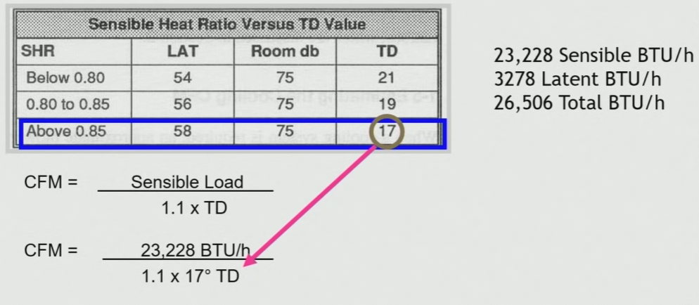
Manual S also has a chart that gives you the evaporator TD based on the SHR of the structure. Pretty handy, right? 

Well, it’s not just for convenience; we need to plug it into a formula.

Determine the CFM for the Structure

We can use the formula below to determine the CFM based on the Manual J load calculation and the TD value derived from the chart in Manual S (with the help of the structure SHR):

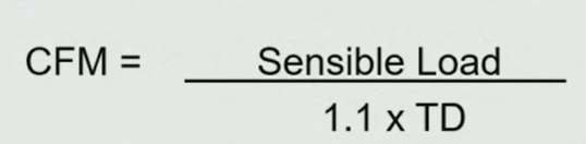
We could simply plug in the numbers: the Manual J load calc’s sensible load and the TD. Ed Janowiak showed an example of this in his symposium presentation from 2022: 

From there, we can select equipment that can deliver the CFM and total, sensible, and latent BTUs as needed according to the Manual J load calculation. We’re not just blindly selecting airflows based on rules of thumb about climate or location (or even structure SHR values, as was recommended in an older edition of Manual J).

What Does That Mean for My Climate?

Long story short, arid climates don’t have to worry about latent loads very much at all when it comes to sizing equipment and setting airflow. The only exception would be if there is a high internal latent load, such as from constant cooking, laundry, showers, and breathing due to a high number of occupants.

In those arid climates, the CFM will also be higher because there’s less of a need to move that air slowly over the coil and get as much moisture to condense on the coil as possible. The structure SHRs will be higher (barring fringe cases with high internal latent loads), so we can achieve those higher airflows and have to worry less about oversizing cooling equipment.

The story is a bit different whenever we get high dew points—either year-round or for at least several months of the year. We must factor latent BTU removal into our load calculations and airflow. Lower fan speeds are more common, usually closer to the outdated Manual J’s 350 CFM rule of thumb. 

However, if you get into the details and follow the entire process laid forth by the ACCA design manuals, you’ll notice that the expanded performance data will show you a trend toward lower fan speeds. But if you go through the entire ACCA design process and do the math, you might still occasionally find some surprises. 

Oh, and if you are in a humid or green-grass market and ever want to size system accessories based on peak dehumidification loads, Manual S can help out with that, too. You just need the dew point, humidity ratio, and mean coincident dry bulb (MCDB) in the Climatic Design Information of ASHRAE’s Handbook of Fundamentals. No more bickering with code officials about peak dehumidification sizing!