This article was written by HVAC contractor and Building Science Whiz, Michael Housh. Thanks, Michael!

For a while, I’ve fallen into this camp where I feel Manual J overshoots heating loads. First off, I would like to say that Manual J is only as good as the information you give it, but we often run into this problem where we have to make educated guesses in the field. Most of us will likely assume insulation values in the wall assemblies (based on age, house type, etc.); windows are often an educated guess (they all suck anyway), and the huge infiltration rate (without a blower door number you’re guessing).

Through some conversations with friends, I was inspired to look at my utility bills and see what knowledge I could gain, and I figured I could take you along for the ride. In my experience, utility companies have a fairly easy way to look at your usage rates for given periods of time. I pulled up my gas usage for 2018 to start slicing and dicing.

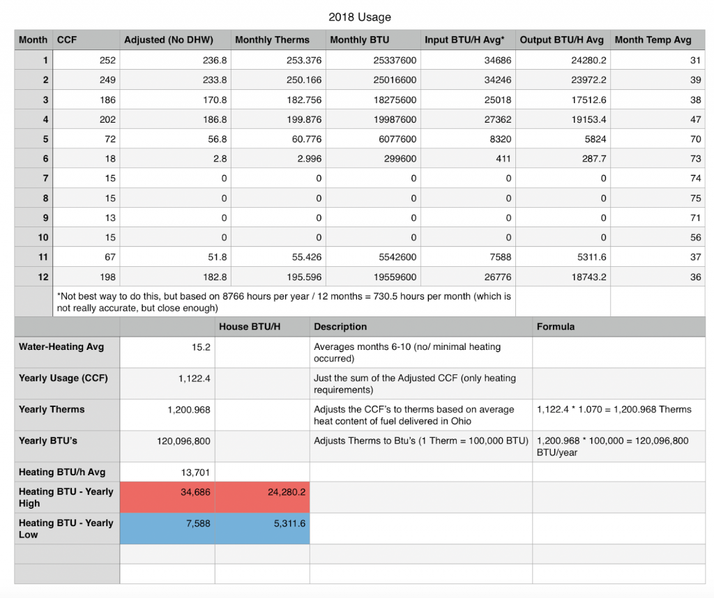
The first thing I did was determine what it costs to heat my domestic hot water by averaging the usage during the summer months, which came out to 15.2 CCF (CCF = volume of 100 cu. ft. of natural gas). I was then able to adjust the data to a usable format, which is the Therm.

1 Therm = 100,000 BTUs. The CCF measurement actually equals a therm if the average heat content of gas is 1,000 BTU in your area. However, national averages are typically higher than that. For where I am in Ohio, our average heat content of gas is 1,070 BTUs per CCF, so I was able to calculate the number of therms used for a given month.

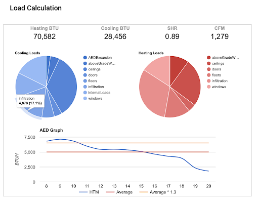
For the sake of brevity, I did a quick generic block load (as I normally would) on just the first floor of my house (which is @ 2400 sq. ft.). I also have some basement area that’s finished, but I haven’t put it into the model yet. I will spare you on the exercise—but the concept is important to understand—that Manual J is rather linear based on outdoor temperature (a good exercise on your own is to generate a load, manipulate the design temperature to several different values and plot them on a graph).

If looking at just usage vs. Manual J, there’s a huge difference. However, my design temperature is 5°, and 2018 was a pretty mild winter, so I looked at the historical weather data for 2018 and added them to my spreadsheet. I also did some calculations (gracefully giving my boiler 70% AFUE) to show the approximate output.

My home was primarily built in the 1950s, with an addition that was likely in the 1980s. For a home of this nature (and especially without a blower door number), I default to “loose” for an infiltration rate. I then took my worst-case month (January). I manipulated the design temperature to 31° in my model, which was the average for that month, and began to adjust the infiltration rate up to “average.” I came out with a pretty similar result to my actual usage.

Once satisfied that the model was pretty close to usage, I set the design temperature back to 5°.

This is a 10-15% difference from the original load/model. Now, all of this stuff is just a little thought experiment I decided to let play out; I hope to expand on these ideas further in the future and hopefully spark some more thoughts on this. DO NOT go out and start doing this, but DO start challenging the norm and come to a deeper understanding for yourself.

—Michael